DMET
Recap of Density Matrix Embedding Theory
Schmidt Decomposition of Wave function
Assume the wave function of the system can be written as: \[\begin{equation} | \psi \rangle = \sum\limits_{i,j} \Psi_{ij} | \psi_i^A \rangle \otimes | \psi^B_j \rangle \end{equation}\]
By implementing Schmidt decomposition, we can get \[\begin{equation} | \psi \rangle = \sum\limits_i \sigma_i | \alpha_i \rangle \otimes | \beta_i \rangle \end{equation}\]
where the \(| \alpha_i \rangle\) and \(| \beta_i \rangle\) are the orthornormally transformed in their own spaces. However, since we usually do not know the full correlated wave function of the system, we can start from the Slater determinant.
The slater determinant can be written as the creation operators on the vacant: \[\begin{equation} | \psi \rangle = \hat c^\dagger_1 \cdots \hat c^\dagger_N | 0 \rangle \end{equation}\]
where \(N\) is the number of electrons. Operating rotations on the occupied orbitals: \[\begin{equation} \tilde c_k^\dagger = \sum\limits_{j=1}^N R_{jk} \hat c_j^\dagger \end{equation}\]
and we can get the rotated Slater determinant: \(| \tilde \psi \rangle = \tilde c_1^\dagger \cdots \tilde c_N^\dagger | 0 \rangle = \det R | \psi \rangle\) Only a phase factor difference to \(| \psi \rangle\).
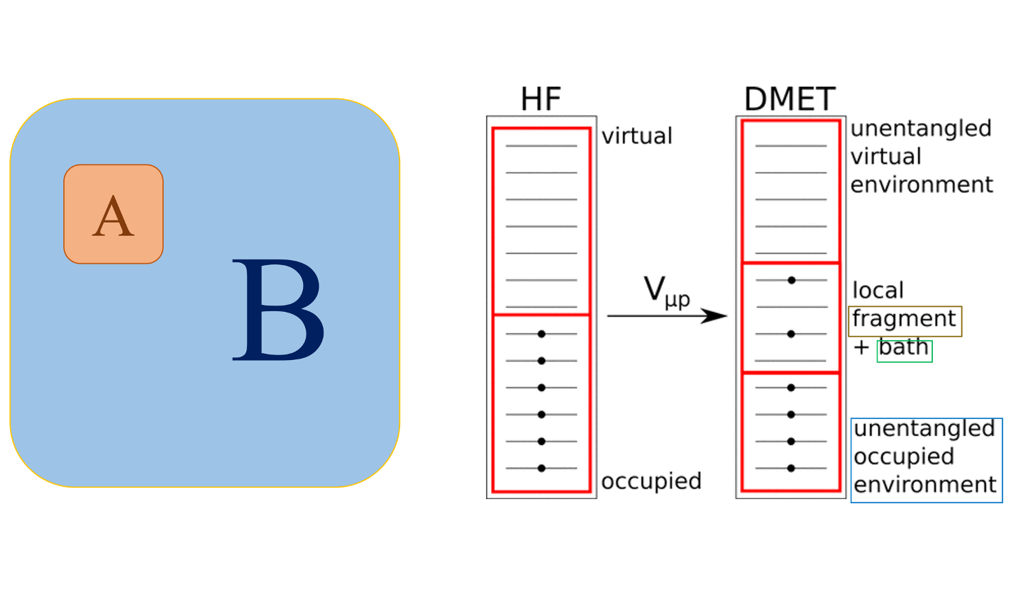
For embedding problems, we'd like to separate the system into "fragment" and "environment", which can be done by localization of the whole sets of molecular orbitals \(\hat a^\dagger_\mu\), which has the relationship \[\begin{equation} \hat c^\dagger_i = \sum\limits_{\mu = 1}^n C_{\mu i}\hat a^\dagger_\mu; \tilde c^\dagger_k = \sum\limits_{\mu = 1}^n \tilde C_{\mu k} \hat a^\dagger_\mu \end{equation}\]
where \(n\) is the number of molecular orbitals (occupied + virtual), and we can find a LO->EO transformation Matrix s.t. \[\begin{equation} \begin{aligned} \tilde C = CR = \begin{bmatrix} P & 0 \\ Q & E \end{bmatrix} \end{aligned} \end{equation}\]
The dimension of \(P, Q, E\) are \(n_A \times n_A,\, n_B \times n_A,\, n_B \times (N - n_A)\), respectively.
Columns of \(P, Q\) and \(E\) are all orthorgonal to each other. In fact it is easy to realize. Considering density matrix \[\begin{equation} \begin{aligned} \rho = \tilde C \tilde C^\dagger = CC^\dagger = \begin{bmatrix} PP^\dagger & PQ^\dagger \\ QP^\dagger & QQ^\dagger + EE^\dagger \end{bmatrix} = \begin{bmatrix} \rho_A & \rho_{AB} \\ \rho^\dagger_{AB} & \rho_B \end{bmatrix} \end{aligned} \end{equation}\]
We diagonize \(\rho_A = U \Gamma U^\dagger\) and then we can choose \[\begin{equation} P = U\Gamma^{1/2},\, Q = (P^{-1} \rho_{AB})^\dagger \end{equation}\]
Since \[\begin{equation} \begin{aligned} I = \tilde C^\dagger \tilde C = \begin{bmatrix}P^\dagger P + Q^\dagger Q & Q^\dagger E \\ E^\dagger Q & E^\dagger E\end{bmatrix} \end{aligned} \end{equation}\]
Then we get \(P^\dagger P = \Gamma, \, Q^\dagger Q = 1 - \Gamma\) and \(Q^\dagger E = 0\).
From \(P. Q\) and \(E\), we can define the new sets of orthonormal creaction operators for each parts: \[\begin{equation} \begin{aligned} \hat c^\dagger_{A, k} = \dfrac{1}{p_k} \sum\limits_{i = 1}^{n_A} P_{ik} \hat a^\dagger_i, k = 1, 2, \cdots, n_A \\ \hat c^\dagger_{B, k} = \dfrac{1}{q_k} \sum\limits_{j = 1}^{n_B} Q_{jk} \hat a_{j+n_A}^\dagger, k = 1, 2, \cdots, n_A \\ \hat c^\dagger_{B, l} = \sum\limits_{j=1}^{n_B} E_{j,l} \hat a_{j+n_A}^\dagger, l = n_A + 1, \cdots, N. \end{aligned} \end{equation}\]
Then the Slater determinant can be written as: \[\begin{equation} \begin{aligned} | \psi \rangle = \prod\limits_{i=1}^{n_A} (p_k \hat c_{A, k}^\dagger + q_k \hat c_{B, k}) \prod\limits_{l = n_A + 1}^{N} \hat c_{B, l}^\dagger | 0 \rangle \\ = \sum\limits_{i_1, \cdots, i_{n_A} \in \{0,1\}} \prod\limits_{k=1}^n p_k^{i_k} q_k^{1-i_k} | i_1 \cdots, i_{n_A} \rangle_A \otimes | 1-i_1, \cdots, 1-i_{n_A}; \Psi_c \rangle_B \end{aligned} \end{equation}\]
So, this result shows that Slater deterninant can be separated to fragment, bath and unentangled parts, where \(n_A\) electrons are allocated to \(2n_A\) fragment+bath orbitals. And the unentangled ones \(|\Psi_c \rangle\) remain doubly occupied.
The alternative way of implementation is to SVD the off-diagonal term \(\rho_{AB}\), then we devide it into \[\begin{equation} \rho_{AB} = U \Gamma V^\dagger = (U \Gamma_p)( \Gamma_q^{\dagger} V^\dagger) = PQ^\dagger , \end{equation}\]
and from the identity \(P^\dagger P + Q^\dagger Q = I\), we have the following identity \[\begin{equation} |\Gamma_p|^2 + |\Gamma_q|^2 = I \end{equation}\]
therefore all the singular value of \(\Gamma\) should \(\in [0, \dfrac{1}{2}]\).
Overview of DMET Algorithm
Embedding Hamiltonian
The single-electron part of Hamiltonian in an embedded space \(A_x + B_x\) is \[\begin{equation} \hat h^x = \sum\limits_{kl}^{\mathrm{frag+bath}} [t_{kl} + \sum\limits_{m,n}^{\mathrm{core}} [(kl|mn) - (kn|ml)] D_{mn}^{\mathrm{env},x}] \hat c_k^\dagger \hat c_l = \sum\limits_{kl}^{\mathrm{frag+bath}} \tilde h_{kl}^x \hat c_k^\dagger \hat c_l \end{equation}\]
Here the notation changes: \(\hat c_k\) are in the fragment+bath space. And the hole embedded Hamiltonian \(\hat H_{emb}^x\) is written as: \[\begin{equation} \hat H_{\mathrm{emb}}^x = \sum\limits_{kl}^{\mathrm{frag+bath}} \tilde h_{kl}^x \hat c_k^\dagger \hat c_l + \sum\limits_{klmn}^{\mathrm{frag+bath}} (kl|mn) \hat c_k^\dagger \hat c_m^\dagger \hat c_n \hat c_l - \mu_{\mathrm{glob}} \sum\limits_r^{\mathrm{frag}} \hat c^\dagger_r \hat c_r \end{equation}\]
Global Chemical Potential and Correlation Potential
The global chemical potential \(\mu_{\mathrm{glob}}\) here is defined to keep the electron in the fragment site (trace of DM block) the same as $n_A$.
In addition, in order to mimic the mean-field wave function and correlated wave function, the determination of mean-field density matrix can be done by adding a correlation 1-electron potential into the mean-field Hartree-Fock: \[\begin{equation} \begin{aligned} \hat C_x = \sum\limits_{kl}^{\mathrm{frag}} u_{kl}^{x} \hat c_k^\dagger \hat c_l \\ \hat F \leftarrow \hat F + \sum\limits_x \hat C_x \end{aligned} \end{equation}\]
the metric of determining \(\hat C_x\) is multiple, and one can use the similarity of 1rdm, i.e. minimizing the penalty function: \[\begin{equation} \mathrm{CF_{full}}(u) = \sum\limits_x \sum\limits_{rs}^{\mathrm{frag+env}(x)} (D_{rs}^x - D_{rs}^{mf}(u)) ^ 2 \end{equation}\]
in which \(D_{rs}^x\) is the density matrix of correlated wave function, and \(D_{rs}^{mf}(u)\) is the density matrix from Hartree-Fock solution with the correlation potential \(\hat C_x\).
However practically, the L2 penalty function may encounter the uncertainty problem. Therefore we provided an alternative way of removing the uncertainty of correlation potential: Assuming that we want to minimize a single-electron Hamiltonian \(\langle \Phi | \hat h | \Phi\) so that \[\forall x, D_{rs}^{mf}(\Phi) = D_{rs}^x\]
and considering that the dual of this problem is convex: \[\begin{equation} \max_{U} \min_{\Phi} \langle \Phi | \hat h | \Phi \rangle + \sum\limits_x \sum\limits_{rs} u_{sr}^x (D_{rs}^{mf}(\Phi) - D_{rs}^{x}) \end{equation}\]
we can work on the dual problem to find optimal \(\{u_{sr}^x\}\). The \(\hat h\) is often chosen as the initial Fock matrix and remain fixed.
Evaluation of DMET Energy
The energy of each fragment: \[\begin{equation} E_x = \sum\limits_{p\in A_x} [\sum\limits_{q}^{\mathrm{frag+bath}} \dfrac{t_{pq} + \tilde h_{pq}^x}{2} D_{qp}^{x} + \dfrac{1}{2} \sum\limits_{qrs}^{\mathrm{frag+bath}}(pq|rs) P_{qp|sr}^x ] \end{equation}\]
which avoids double counting of unentangled contribution to each fragment, and therefore the total energy is the summation of different parts: \[\begin{equation} E = E_{\mathrm{nuc}} + \sum\limits_x E_x \end{equation}\]
In a nutshell, DMET approximates the total energy from the correlation energy of each parts.
Details
Embedding-space Hamiltonian
If we do a partial trace on the total Hamiltonian $\hat H$, for 1-electron hamiltonian, we have \[\begin{equation} \langle \Psi_c | \hat H_1 | \Psi_c \rangle = \sum\limits_{KL}^{\mathrm{frag+bath}} t_{KL} \hat a^\dagger_K \hat a_L + \sum\limits_{PQ}^{\mathrm{core}} D_{PQ}^{\mathrm{core},x} t_{PQ} \end{equation}\]
and on 2-electron Hamiltonian, only [core*4]{.title-ref}, [emb*4]{.title-ref} and [core*2+emb*2]{.title-ref} contribution are conserved, thus we have \[\begin{equation} \begin{aligned} \langle \Psi_c | \hat H_2 | \Psi_c \rangle = \dfrac{1}{2} \sum\limits_{PQRS}^{\mathrm{emb}} g_{PQRS} \hat a^\dagger_P \hat a^\dagger_R \hat a_S \hat a_Q \\ + \sum\limits_{PQ}^{\mathrm{emb}} \sum\limits_{RS}^{\mathrm{core}} (g_{PQRS} - g_{PSRQ}) D_{RS}^{\mathrm{core}, x} \hat a^\dagger_P \hat a_Q \\ + \dfrac{1}{2} \sum\limits_{PQRS}^{\mathrm{core}} g_{PQRS} \Gamma_{PQRS} \end{aligned} \end{equation}\]
here the capitalized letters are spin-orbital indices. Thus the effective embedding hamiltonian (without constants totally contributed by core) is: \[\begin{equation} \begin{aligned} \langle \Psi_c | \hat H | \Psi_c \rangle = \sum\limits_{PQ}^{\mathrm{frag+bath}} (t_{PQ} + \sum\limits_{RS}^{\mathrm{core}} (g_{PQRS} - g_{PSRQ}) D_{RS}^{\mathrm{core}, x}) \hat a^\dagger_P \hat a_Q \\ + \dfrac{1}{2} \sum\limits_{PQRS}^{\mathrm{emb}} g_{PQRS} \hat a^\dagger_P \hat a^\dagger_R \hat a_S \hat a_Q \end{aligned} \end{equation}\]
Democratic Partitioning
Considering the representation in EO basis, the impurity index in \(x\), the fragment space is \(A_x\), the bath space is \(B_x\), and the core/vir space is \(C_x\), then the one-electron democratic partition energy is \[\begin{equation} \begin{aligned} E_{1,PQ} = \dfrac{1}{2} \langle \Psi | t_{PQ} \hat a^\dagger_P \hat a_Q + t_{QP} \hat a^\dagger_Q \hat a_P | \Psi \rangle = \begin{cases} \dfrac{1}{2} (t_{PQ} D_{PQ} + t_{QP} D_{QP} ), Q \in A_x + B_x; \\ 0, Q \in C_x \end{cases} \end{aligned} \end{equation}\] \[\begin{equation} \begin{aligned} E_{2,PQRS} = \dfrac{1}{8} \langle \Psi | g_{PQRS} \hat a^\dagger_P \hat a^\dagger_R \hat a_S \hat a_Q + g_{QPRS} \hat a^\dagger_Q \hat a^\dagger_R \hat a_S \hat a_P + g_{QRPS} \hat a^\dagger_Q \hat a^\dagger_P \hat a_S \hat a_R + g_{QRSP} \hat a^\dagger_Q \hat a^\dagger_S \hat a_P \hat a_R| \Psi \rangle \\ = \begin{cases} \dfrac{1}{8} (g_{PQRS} \Gamma_{PQRS} + \cdots) , QRS \in A_x + B_x , \\ \dfrac{1}{8} (g_{PQRS} D_{RS} D_{PQ} + g_{QPRS} D_{QP} D_{RS} - g_{QRSP} D_{QP} D_{SR}), RS \in C_x ; \\ \dfrac{1}{8} (-g_{PQRS} D_{RQ} D_{PS} + g_{QRPS} D_{QR} D_{PS} + g_{QRSP} D_{QR} D_{SP}), QR \in C_x; \\ -\dfrac{1}{8} (g_{QPRS} D_{QS} D_{RP} + g_{QRPS} D_{QS} D_{PR}), QS \in C_x . \end{cases} \end{aligned} \end{equation}\]
After the rearrangement of the index, we can get the representation of democratic-partition result for index \(P \in A_x\): \[\begin{equation} \begin{aligned} E_{P} = \mathrm{Re} \sum\limits_{Q}^{A_x + B_x} (t_{PQ} + \sum\limits_{RS}^{C_x} \dfrac{1}{2} (g_{PQRS} - g_{PSRQ}) D_{RS}) D_{PQ} \\ + \dfrac{1}{2} \sum\limits_{QRS}^{A_x + B_x} g_{PQRS} \Gamma_{PQRS} \end{aligned} \end{equation}\]
which corresponds to the Eq.(28) in Practical guide. Here the density matrices are the \(\langle \Psi_x | \cdots | \Psi_x \rangle\) if the indices are in the embedding space, and \(\langle \Psi_c | \cdots | \Psi_c \rangle\) if the indices are in the core space.
In general case, if the two wave-functions share the same core but with the different embedding-space part, then the result of "democratic-partition energy" is written as: \[\begin{equation} \begin{aligned} E_P = \dfrac{1}{2} \sum\limits_{Q}^{A_x + B_x} (t_{PQ} + \sum\limits_{RS}^{C_x} \dfrac{1}{2} (g_{PQRS} - g_{PSRQ}) D_{RS}) D_{PQ} + \dfrac{1}{4} \sum\limits_{QRS}^{A_x + B_x} g_{PQRS} \Gamma_{PQRS} \\ + \dfrac{1}{2} \sum\limits_{Q}^{A_x + B_x} (t_{QP} + \sum\limits_{RS}^{C_x} \dfrac{1}{2} (g_{QPRS} - g_{QSRP}) D_{RS}) D_{QP} + \dfrac{1}{4} \sum\limits_{QRS}^{A_x + B_x} g_{QPRS} \Gamma_{QPRS} \end{aligned} \end{equation}\]
in which we regard to \(\langle \Psi_x | \cdots | \Psi_y \rangle\) when we talk about \(D_{PQ}\) and \(\Gamma_{PQRS}\) etc.
Define the effecitve one-electron Hamiltonian \[\begin{equation} \tilde t_{PQ} = t_{PQ} + \sum\limits_{RS}^{C_x} \dfrac{1}{2} (g_{PQRS} - g_{PSRQ}) D_{RS} \end{equation}\]
if we try to start from Fock matrix \[\begin{equation} f_{PQ} = t_{PQ} + \dfrac{1}{2} \sum\limits_{RS}^{A_x + B_x + C_x} (g_{PQRS} - g_{PSRQ}) D_{RS} \end{equation}\]
then the effective one-electron Hamiltonian \[\begin{equation} \tilde t_{PQ} = f_{PQ} - \dfrac{1}{2} \sum\limits_{RS}^{A_x + B_x} (g_{PQRS} - g_{PSRQ}) D_{RS} \end{equation}\]
then we can write the democratic-partition energy as the form of evaluating some "weighted Hamiltonian" with the density matrices within the embedding space: \[\begin{equation} \sum\limits_P^{A_x} E_P = \sum\limits_{PQ}^{A_x + B_x} \tilde t_{PQ} w_{PQ} D_{PQ} + \dfrac{1}{2} \sum\limits_{PQRS}^{A_x + B_x} g_{PQRS} W_{PQRS} \Gamma_{PQRS} \end{equation}\]
in which the weights are: \[\begin{equation} \begin{aligned} w_{PQ} = \dfrac{1}{2} n_{A_x} (PQ); \\ W_{PQRS} = \dfrac{1}{4} n_{A_x} (PQRS). \end{aligned} \end{equation}\]
where \(n_{A_x} (PQRS)\) is the number of index within \(A_x\) among \(P,Q,R\) and \(S\).